Kevin T. Kilty
Copyright © 1989,1999 All Rights Reserved
The purpose of this paper is to discuss data smoothing and filtering and its use in processing geophysical data. While most of my examples deal with removing cultural noise from ground magnetic data, spatial filtering applies to other noise processes and other types of data. For example, spatial filtering includes linear transformations of potential fields of data, or high-pass filtering of drill hole data to produce a residual structure map.
Filtering or smoothing can be done in the space domain, an example is the running average filter; or, in the wavenumber domain, as is typically the case with analytic continuation. Whether filtering is done in the wavenumber domain or in the space domain, obtaining an accurate estimate of the spectrum of the data is a prerequisite concern. There are three items to consider in this regard. In order they are (1) the effects of aliasing, (2) the effects of using a finite length data window, and (3) the effects of noise. In the wavenumber domain an additional concern is the use of an FFT algorithm to calculate the spectrum. I will discuss each topic separately.
Aliasing Aliasing in the collection of spatial data differs from aliasing in the collection of time series (seismic data) in one important respect. Because time series are sampled continuously in time, one may eliminate aliasing to any desired degree by applying an electronic filter to the signal prior to digital conversion. Spatial data, on the other hand, are collected at isolated locations and immediately suffer some degree of aliasing. Not all spatial data suffer aliasing to the same degree however. For example, drill hole data represent very small, discrete samples and one must assume that such data might be badly aliased. Magnetic data, on the other hand, are sometimes collected on the ground using the average value of readings taken in a starlike pattern, or in the air using a moving sensor that has a finite integration time. Either method acts as an anti-aliasing filter. In addition magnetic and other potential fields data obtain some anti-aliasing whenever there is substantial depth to the source of an anomaly. The smoothing of a potential field with distance from the source is itself a filtering operation.
There is a belief (expressed in the literature) that digitizing a contour map or profile, or resampling digitized data for purposes of modeling is equivalent to low-pass filtering. This is not so. While the spectrum of digitized data displays no energy above the Nyquist frequency, digitizing has not filtered the data. It moves energy around in a spectrum in a way no filter would. If digitizing or resampling is done without providing some anti-aliasing then aliasing occurs in addition to that which occurred in the original field measurements.
The effect of aliasing is generally easy to describe. Aliased potential fields are too smooth. Interpretation of this data places sources of the field too deep. However, aliasing has other, more interesting effects. It may cause a subtle feature to be removed when it should have been retained in a residual. Even more interesting is the production of phantom patterns in an image. Moire patterns, for example, result from aliasing a periodic spatial image.
Aperture Spatial data are collected and analyzed over finite intervals, whereas the fields themselves extend over all space. A restricted data window length (aperture) has an effect on the data spectrum described approximately as follows.
The finite window of data is the product of the actually unbounded data and a window of finite length and unit height. The spectum of the window of data is therefore the convolution of the actual data spectrum with the spectrum of the window or aperature. In the specific case of a rectangular aperture, the aperture spectrum is a SINC function which has a dominate primary peak at zero lag and secondary peaks at multiples of the inverse aperture length. Thus, any sharp peak that exists in the actual data spectrum is observed as a central dominant peak surrounded by a family of secondary peaks. Closely spaced peaks in the actual spectrum may become difficult to resolve from one another in the observed spectrum. Obviously a longer data window leads to better resolution of closely spaced anomalies. Data length plays a role analogous to that of aperture in optics1.
In order to improve the resolution of finite length data, one may use windows having shapes more smooth than the rectangular window. This will smooth the spectrum. Common window shapes are the Bartlett window (rectangular taper), the Tukey window (cosine taper), and the Parzen window (cubic polynomial taper). While applying these windows does smooth the spectrum, it unfortunately causes the spectrum to be biased since the tapering will discount information at the edges of the window. In geophysical applications one is always a little short of data anyway and would like not to discount any information. In this case we extrapolate our data beyond the observations in some reasonable way and apply a window to this data that has a unit amplitude over the actual data and tapers to zero within the extrapolated region. Upon reconstructing the space domain data after filtering we can remove the extrapolated regions.
If course, this method still biases the spectrum. But the bias is largely the result of our assumptions, and not the result of how the data are distributed. I have found this method to work very well.
Noise Noise is related to aliasing and aperture. It is generally a high wavenumber process. If data are aliased, however, noise can become mixed with the signal at low wavenumbers. In extreme cases it becomes the signal. Noise within a finite data window reduces the resolution of our data even when it is not aliased. Noise is a particular concern in environmental applications of geophysics because the surveys are conducted in populated areas that are especially prone to noise. Powerlines, buried drums, pipes, and fences all serve to obscure geological signals. My approach to the problem of noise is to filter or smooth the data, which is the subject of this paper.
Many filters are defined entirely by the process they are meant to perform. For example, analytic continuation or reduction to pole defines a precise form for a filter for all wavenumbers. Pure spatial filters, however, are not precisely defined. We are free to design a filter that best accomplishes our goal. Generally the goal is to separate a geological signal from noise or to separate interfering geological signals from one another. Sometimes this is an impossible task. It is not possible to separate noise and signal, or two signals, that share space in the spectrum. If spectra overlap significantly, filtering is not a solution.
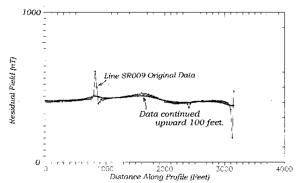
Figure 1 shows a ground magnetic profile collected on the flank of a magnetic anomaly from a diabase intrusive. The anomaly of interest lies between 500 feet and 2500 feet on the profile. It is obscured mildly by 4 short-wavelength, high amplitude anomalies from cultural objects. There are several approaches to removing this noise. First, examine the spectrum of the data.

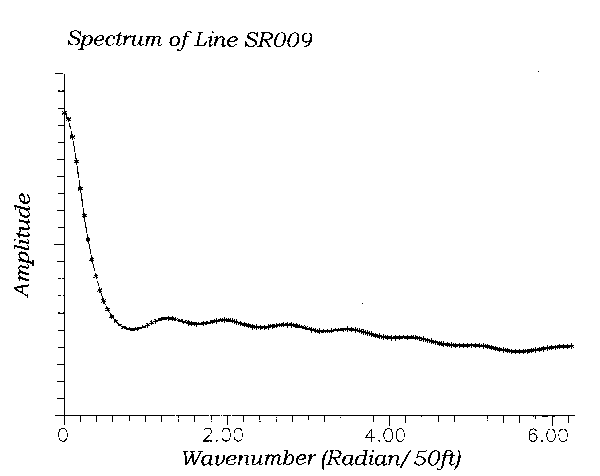
Figure 2 shows the data spectrum calculated with a Burg algorithm. The signal manifests itself as the spectral peak near zero wavenumber. Surprisingly, the noise spikes do not appear distinctly in the spectrum at all. They are represented by the subtle, broad spectral peak from 1.0 to 3.0 radians/50ft. The breadth of this peak is an illustration of the principal that brief spatial events have a broad spectrum and visa-versa. Because of the breadth and subtlety of the noise spectrum, we cannot design a linear filter to remove it unless the filter has a sharp response near zero wavelength. So, for example, a running average filter, which has broad response will not work. What we seek is a de-spiking filter.
An obvious approach is to draw a smooth curve through the data by hand. This approach is possible in this case only because the noise is so distinctly different from the signal. More typically the noise would be randomly distributed and more dense. Smoothing by hand in such situations often leads to clusters of noisy points becoming smoothed into phantom signals, and thus works no better than does calculating a running average.
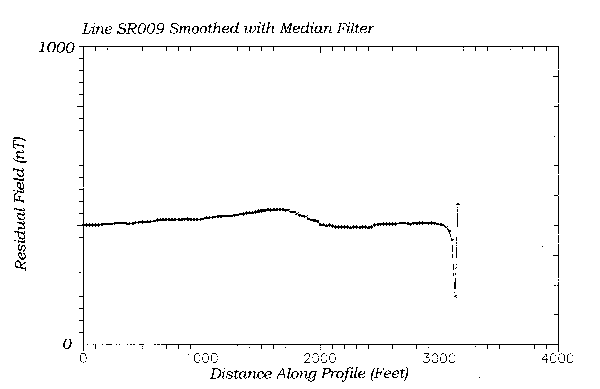
A particularly useful de-spiking filter is the running median filter. Several efficient algorithms for computing a running median are available in the literature (Evans, 1982). Figure 3 shows the result of passing our magnetic profile through an 11 point running median filter. The noise spikes are removed completely, without altering the shape of the anomaly of interest. This is an important consideration. If our filtering operation distorts the shape of an anomaly, it obviously affects any interpretation we make through modeling.
One question we would like to answer is how are we distorting our signal in the process of smoothing. The running average filter is easy to analyze in this regard. It, and any similar low pass filter, tends to increase the apparent depth of the source. Thus, models constructed from data smoothed with a low-pass filter will tend to be too deep. Moreover, most low-pass smoothing tends to move shallow sources much further than deep sources. Thus, if the data contain useful information on the vertical distribution of sources or the shape of a source, that information is distorted or lost completely with smoothing.
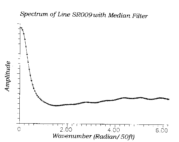
The effect of a de-spiking running median, on the other hand, is difficult to characterize. Its behavior depends on the data. In some respects it behaves like a low-pass filter. I demonstrated this behavior in my example. However, it is possible to get a short-wavelength but persistent sinusoid to pass through a running median, and sharp signal transitions, clock pulses for instance, can pass through it unaltered. Thus, the running median is not really a low-pass filter. Also, a running median filter may actually increase the high-wavenumber noise while it eliminates spikes. Figure 4 for example shows the spectrum of line #9 computed after application of the running median filter. As shown, the high-wavenumber noise level has increased even as noise in the range of 1.0-3.0 rad/50ft. has decreased.
One low pass filter that provides smoothing but which does not distort models made from the smoothed data is analytic continuation away from the source. I will refer to this as upward continuation, as is the custom in geophysics. But because sources may be simultaneously above and below our profile, it is more accurately called continuation away from the source. Analytic continuation away from a source is a low-pass filter. It is purely a calculation of what the field would look like at a greater distance from the source. It does not distort the shape of any model fitting the data, but it does reduce resolution by virtue of placing our observations further away.
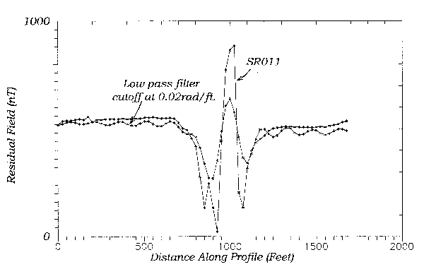
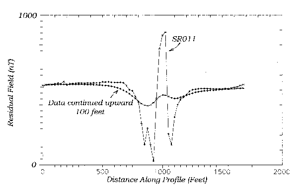
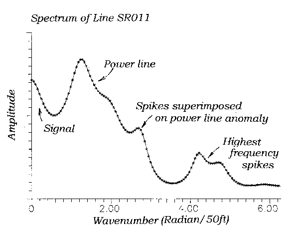
In Figure 5 I show a magnetic profile taken beneath a power line. There is a large positive anomaly at 1000 feet, with flanking negative lobes, that corresponds to the power line. This anomaly completely obscures an anomaly from a diabase intrusive. In fact, the only indication of the intrusive is that the magnetic intensity appears on the left side of the profile at a higher value than on the right. Continuation of the data 100 feet away from the source is shown in Figure 6. The power of continuation to smooth data is apparent in this figure. Unfortunately the anomaly of the power line still dominates the profile. Figure 7 shows a power spectrum calculated from the raw data. The spectrum is dominated by the power-line anomaly, as shown by the large spectral peak near 1.4 rad/50 ft. Our signal is represented by the small peak near zero. An approximate rule states that two features are not separable by filtering if they are not distinct on a spectrum at their half-power points. Since our signal and the power-line anomaly are distinct only at the .75 power point they probably cannot be separated from each other. At least I have not found any filter that can do this. My only recourse in this case is to use what information is available -- the difference in magnetic intensity between the left and right side.
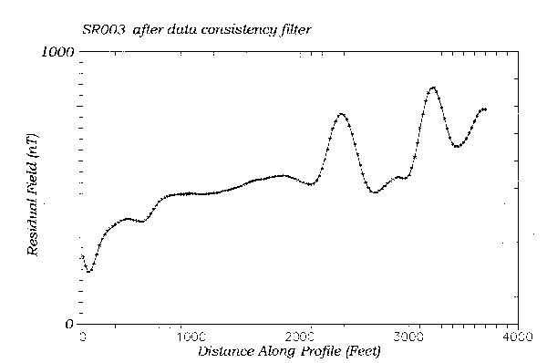
To this point I have discussed filtering only as it applies to the smoothing of data without indicating any design criteria or any criteria by which a filter is measured. In most cases these are dictated by preconceptions the geophysicist has about his target. However, one interesting approach to this problem which is not well known among geophysicists is smoothing for data consistency. This concept is borrowed from spectroscopy (Hayden, 1987), but it applies equally well to geophysical measurements.
By consistency I mean that our data should be free of features not resolvable by an instrument. In geophysics it is distance between the source and instrument which renders some features not resolvable. For example, we measure a magnetic profile on the ground surface, and find that it is corrupted by measurement noise and nearby cultural sources which are uncorrelated or only weakly correlated from one measurement to the next. The signal of interest, however, is from a more distant source and appears on many adjacent measurements. Suppose we know that the source we are interested in cannot be closer than, say, 100 feet to the ground surface. We can design a filter that excludes any features in our profile that cannot have come from a source 100 feet or more away. To do this we use the upward continuation filter applied iteratively according to the following prescription.
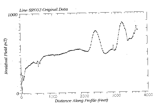
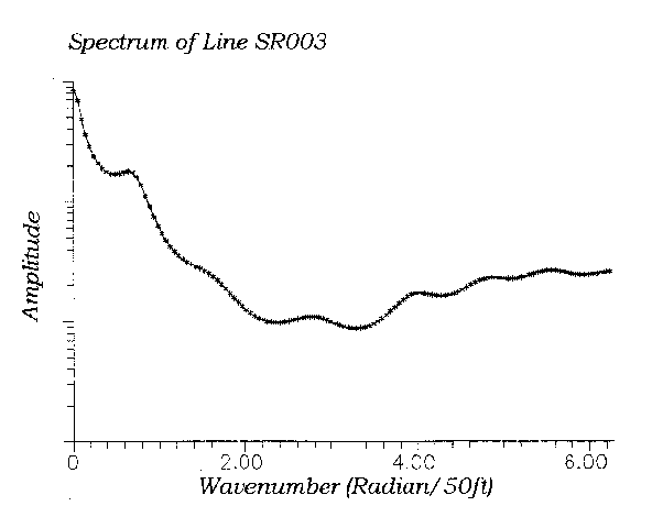
Figure 8 shows a magnetic profile that contains anomalies of
geological origin and some added measurement noise. Its spectrum is
shown in Figure 9. The spectrum has a peak value near zero wavenumber,
which is contributed by the linear increase from left to right and the
low amplitude sinusoid, and a second peak at 0.8 rad/50ft. which results
from two obvious humps in the profile. Beyond this there is only a
Using an FFT for filtering involves special considerations. First, an FFT requires evenly spaced data. Sometimes data are collected on an evenly spaced grid. However, data are sometimes more advantageously collected on an uneven spacing. In order to use an FFT with unevenly spaced data, one must first grid the data. This links a spectral estimate with the performance of a gridding algorithm.
Using an FFT algorithm for the calculation of the spectrum has a further effect. The calculation involves an implicit assumption that the data as represented in the map or profile are periodic with period Lx in the x direction and Ly in the y direction, where L is the data window length. The most apparent result of this assumption is that the spectrum is no longer continuous but defined at wavenumbers that are a multiple of 2ă/L, and thus, has the appearance of a Fourier series. However, the coefficients calculated from the fast Fourier transform are not a Fourier series truncated at the Nyquist frequency, but are instead the coefficients of a trigonometric interpolator. This is s an aliased Fourier series.
The use of an FFT also alters the true spectrum of the data in another way. If the opposite edges of the map do not have the same amplitude, or if any derivatives of the data are discontinous, the periodic discontinuity seen by the FFT will manifest itself in Gibbs oscillations and ficticious power, especially in the high wavenumber part of the spectrum. This ficticious power is needed to recreate the discontinuity at the map edge in an inverse transformation. Hence, if a filtering process alters the high wavenumber part of the spectrum, the discontinuity will become distributed through the map. In particular, if the filtering removes the high wavenumber part of the spectrum (upward continuation), one will notice the discontinuity diffusing into the map from the edges. This is not a desirable situation, but even worse is the effect that amplification (downward continuation) of the high wavenumber part of the spectrum has. In this case the ficticious power dominates the entire map. The process of apodization, described in the section on aperture and in the trailing notes, is a means of mitigating the worst effects of the discontinuities since it tends to eliminate the discontinuity between opposite map edges.
Notes
1. The analogy with optics can be taken further, the process
equivalent to smoothing the aperture in optics is
called apodization, which means literally to remove the feet.
2. Stewart Sandberg, who is now a professor of geology at the University of Southern Maine,
contributed data to this paper.